In Part 1, I introduced the problem of rudder position sensing for SCANS and explained why Gray code (and optical sensing) provides reliable absolute position encoding in the presence of mechanical imperfection and electrical noise. This second part examines the first part of the implementation: the translation of Gray code theory into manufacturable encoder disk. The central challenge was not in the mathematical abstraction of Gray code—that’s been understood since the 1940’s—but in the practical synthesis of a physical disk that satisfies multiple competing constraints: manufacturability via fused deposition modeling, reliable optical readability, mechanical robustness, and geometric compatibility with the mounting hardware. The solution required developing a parametric design system that could navigate these constraints systematically.
Physical Constraints and Design Requirements
Fused deposition modeling (FDM) has fundamental limits on minimum feature size determined by nozzle diameter. Optical sensors require minimum feature dimensions for reliable discrimination between transmissive and opaque regions. The encoder disk must possess sufficient structural integrity to resist warping and mechanical stress. Additionally, inside a housing containing the reader, and electronics with geared linkage to the rudder post.
The 256-position, full-rotation encoder described in Part 1 represents one point in a larger design space. A more robust approach required a parametric generator capable of producing valid encoder geometries across a range of specifications: varying position counts, alternative arc angles (for partial-rotation applications), different radial dimensions, and adjustable resolution requirements. Rather than implementing a single fixed design, I developed software that encodes the mathematical relationships between parameters, validates configurations against manufacturing constraints, and performs automated optimisation using a genetic (evolutionary) algorithm.
Mathematical Foundation
The system’s foundation rests on the Gray code conversion algorithm. For any position $n$ in the range $[0, N-1]$ where $N$ represents the total position count, the Gray code value is computed through the exclusive-OR operation:
$$\text{Gray}(n) = n \oplus (n \gg 1)$$
This bitwise XOR operation between the position value and its right-shifted counterpart produces the single-bit-change property characteristic of Gray code. To generate physical track patterns, individual bits must be extracted from this encoded value.
For an $m$-bit Gray code, where $m = \lceil \log_2(N) \rceil$ represents the minimum number of tracks required, each position encodes as $m$ binary digits. Bit extraction follows:
$$\text{bit}_i = \left(\lfloor\frac{\text{Gray}(n)}{2^i}\rfloor\right) \bmod 2$$
where $i \in [0, m-1]$. This operation corresponds to (gray_value >> i) & 1 in implementation.
For an in depth discussion of Gray Code, it’s theory, history, and uses, please see: https://en.wikipedia.org/wiki/Gray_code
These extracted bits map to concentric physical tracks on the encoder disk. The track assignment follows a specific convention: Track 0 (outermost radius) carries the least significant bit (LSB), while Track $m-1$ (innermost radius) carries the most significant bit (MSB). This radial ordering derives from optical considerations rather than arbitrary choice.
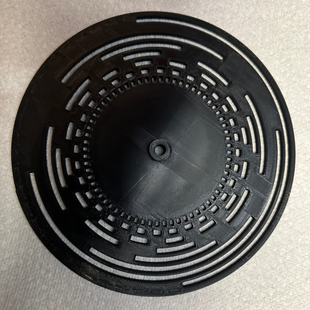
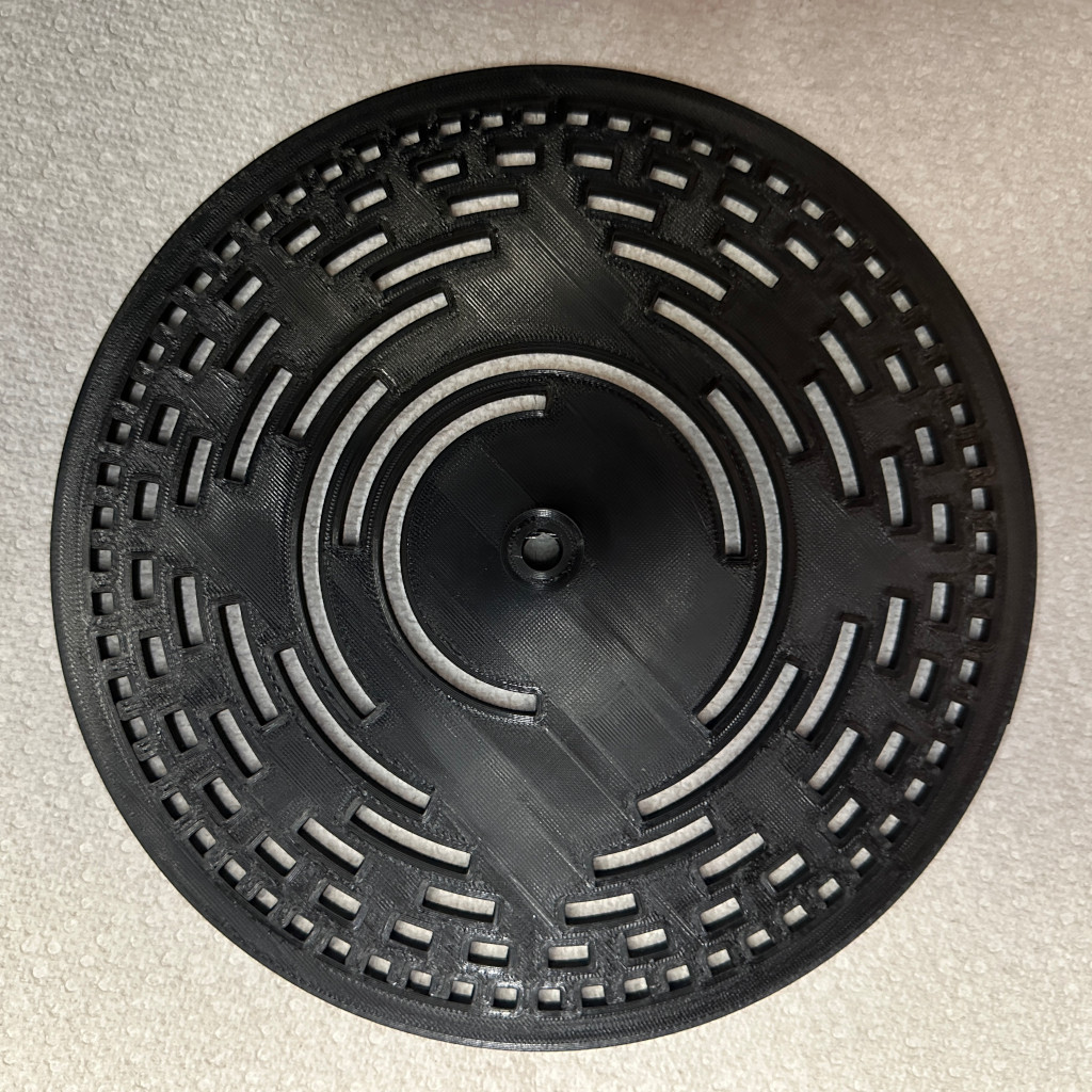
The LSB exhibits the highest transition frequency—approximately every other position—as the encoded sequence increments. Positioning this bit on the outermost track maximizes the arc length of each segment, improving optical sensor reliability. The MSB transitions least frequently (once per half-cycle of the full sequence), making the shorter arc lengths of inner tracks less problematic for detection.
The conversion from bit patterns to physical geometry requires determining the spatial distribution of transmissive regions on each track.
Track Layout and Geometric Constraints
Each track occupies an annular sector—a ring segment defined by inner radius, outer radius, and angular extent. For a disk with outer radius $R_{\text{outer}}$ and inner radius $R_{\text{inner}}$ (determined by the mounting hole diameter), tracks are positioned sequentially from the outer edge inward with spacing between adjacent tracks.
Given $m$ tracks with uniform track width $w$ and inter-track spacing $s$, the track pitch $p$ (center-to-center distance) becomes:
$$p = w + s$$
Track $i$, indexed from 0 at the outermost position, occupies radial bounds:
$$R_{\text{outer},i} = R_{\text{outer}} – i \cdot p$$
$$R_{\text{inner},i} = R_{\text{outer},i} – w$$
A fundamental geometric constraint requires that the innermost track not extend below the inner mounting radius:
$$R_{\text{inner},m-1} \geq R_{\text{inner}}$$
This inequality establishes an upper bound on the number of tracks that can be accommodated within the available radial space. The usable radial dimension equals $R_{\text{outer}} – R_{\text{inner}}$, while the radial space required for $m$ tracks totals $m \cdot w + (m-1) \cdot s$. Violation of this constraint triggers validation errors in the parameter checking system.
Translating Bit Patterns to Physical Cutouts
The conversion from bit patterns to physical geometry requires determining the spatial distribution of transmissive regions on each track. In a transmissive optical encoder, a ‘1’ bit indicates light transmission through a cutout or slot, while a ‘0’ bit indicates light blockage by solid material.
For each track, the bit pattern across all $N$ positions forms a binary sequence: $[b_0, b_1, b_2, \ldots, b_{N-1}]$ where $b_i \in \{0, 1\}$. Rather than generating individual cutouts for each ‘1’ bit, the algorithm identifies maximal contiguous subsequences of ‘1’ values and creates a single continuous aperture spanning the corresponding angular range. This approach reduces geometric complexity and improves manufacturing reliability.
For positions distributed over arc angle $\theta_{\text{arc}}$, each position corresponds to angular increment:
$$\Delta\theta = \frac{\theta_{\text{arc}}}{N}$$
A contiguous run of $k$ consecutive ‘1’ bits beginning at position $p$ generates a cutout spanning the angular interval $[p \cdot \Delta\theta, (p + k) \cdot \Delta\theta]$. To ensure complete material removal through the disk thickness, the implementation adds a small angular overlap (typically 0.1°) at each boundary and extrudes the cutout to height slightly exceeding the nominal disk thickness.
Geometric primitives are constructed using SolidPython, a Python library providing programmatic generation of OpenSCAD code. Each cutout represents an extruded polygon—specifically, the closed path defining an annular sector. Sector boundary points are computed by parametric generation of arc segments at both inner and outer radii.
For an arc spanning angles $\theta_1$ to $\theta_2$ at radius $R$:
$$x(\theta) = R \cos(\theta)$$
$$y(\theta) = R \sin(\theta)$$
with $\theta$ interpolated over 50 or more discrete steps to achieve smooth curve approximation. The outer arc points are concatenated with reversed inner arc points to form a closed polygon suitable for extrusion.
Manufacturing Constraints in Fused Deposition Modeling
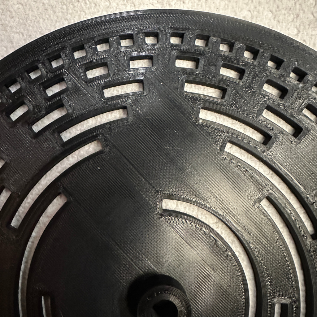
FDM works by extruding thermoplastic through a heated nozzle, with typical diameters of 0.4mm for standard applications or 0.2mm for precision work. 0.4mm is usually preferred as smaller nozzle diameters are increasingly prone to clogging as the diameter decreases. The nozzle diameter is a lower bound on achievable feature dimensions and the minimum feature width– for a 0.4mm nozzle–is approximately 0.8mm and features below this become unreliable Inter-feature gaps present similar constraints: insufficient gap width permits unintended bridging where extruded material spans the gap, occluding what should be transmissive.
The critical parameters affecting manufacturability are gap width (expressed in angular measure) and inter-track spacing. Gap width $\theta_{\text{gap}}$ determines each cutout’s angular span. At radius $R$, this angular measure translates to linear dimension:
$$d_{\text{gap}} = \frac{\theta_{\text{gap}} \cdot \pi \cdot R}{180}$$
This gap must exceed minimum thresholds to reliably separate adjacent solid regions. The software incorporates a printability analyzer that evaluates these constraints across all tracks, generating warnings when features approach or violate minimum dimensional thresholds.
A fundamental tension exists between these constraints and design objectives: larger gaps and spacing enable more reliable manufacturing but consume radial space, reducing the number of tracks that fit within available dimensions and thereby limiting resolution. Conversely, aggressive dimensional reduction permits higher track counts and resolution but risks manufacturing failures. This multi-objective optimization problem, involving competing constraints and nonlinear relationships between parameters, motivates the application of evolutionary search algorithms.
Evolutionary Optimisation of the Parameter Space
Rather than manual parameter tuning through iterative trial and error, I implemented a genetic algorithm to perform systematic search of the design space for near-optimal configurations. The algorithm represents each candidate encoder design as a “genome”—a vector of parameter values completely specifying the disk geometry and encoding characteristics.
The evolutionary process begins with a population of randomly generated genomes, typically 30 to 50 individuals representing diverse points in the parameter space. Each genome undergoes evaluation via a multi-objective fitness function scoring performance across several criteria:
- Printability (weighted at 40% of total fitness) assesses manufacturability by evaluating minimum feature sizes, gap widths, track spacing, and wall thicknesses against FDM constraints. Designs violating printability requirements receive substantial fitness penalties, effectively steering the population toward manufacturable solutions.
- Resolution (20% weight): quantifies the encoder’s ability to distinguish discrete positions. Higher position counts generally improve angular resolution, though with diminishing returns beyond certain thresholds and subject to physical size constraints.
- Encoding efficiency (20% weight): measures Gray code utilisation relative to track count. For $m$ tracks supporting up to $2^m$ distinct codes, using exactly a power-of-two position count (e.g., 32 positions with 5 tracks) achieves 100% efficiency. Configurations using fewer than $2^m$ positions exhibit lower efficiency due to unused code space.
- Size optimisation (10% weight): rewards designs approaching the target outer diameter. Significant deviation either direction indicates suboptimal space utilization or geometric incompatibility with mounting constraints.
- Manufacturability (10% weight): captures secondary considerations including preference for standard dimensional values, reasonable arc angles, and design simplicity affecting assembly and optical alignment.
The fitness function computes a weighted sum of these normalised component scores, with a 20% multiplicative bonus applied to genomes satisfying all validation constraints. Invalid parameter combinations receive zero fitness, eliminating them from reproduction.
Evolution proceeds through tournament selection, where small randomly-chosen subsets compete and the highest-fitness individual from each tournament becomes a parent for the next generation. Elitism preserves the top 10% of each generation unchanged, preventing loss of high-quality solutions. Remaining positions in the next generation are filled by offspring generated through crossover and mutation operations.
Crossover combines parental genomes by randomly inheriting each optimisable parameter (track width, track spacing, gap width) from one parent or the other. Mutation subsequently introduces variation through bounded random perturbations, typically ±20% of current values, with parameter-specific range constraints preventing physically impossible values.
A critical feature permits fixing certain parameters while optimising others. For the rudder encoder application, mounting geometry dictates outer diameter, inner diameter, and arc angle as fixed constraints determined by mechanical requirements. The algorithm holds these constant while optimising the track layout parameters governing optical performance and manufacturability. This constrained optimization focuses computational effort on the actual degrees of freedom in the design problem.
The algorithm executes for a complete generation count—typically 50 generations—without implementing early termination criteria. This ensures thorough exploration of the parameter space rather than premature convergence to local optima. Empirical observation indicates that novel high-quality solutions often emerge in later generations as the population converges toward optimal regions of the search space.
Application of the genetic algorithm to the encoder specifications yielded a best-fitness solution of 1.115 after 50 generations. The optimized parameter set comprises 32 positions (5-bit Gray code), 116.2mm outer diameter, 35.6mm inner diameter, 57.1° arc angle, 3.3mm track width, 1.7mm track spacing, and 2.8° gap width. These values replaced the initial hand-tuned parameters as the system’s default configuration.
Software Architecture
The software discussed in this article is freely available (MIT license) at: https://github.com/susannecoates/gray-encoder-disk-generator
For information and discussion on the software architecture and instructions on how to use it, please see the Wiki: https://github.com/susannecoates/gray-encoder-disk-generator/wiki
Discussion
While Gray code’s theoretical properties are well known, addressing additive manufacturing limitations, optical sensor characteristics, mechanical tolerances, and the complex interactions between geometric parameters proved to be an interesting challenge. The genetic algorithm, initially, was a computational convenience—a method to avoid manual parameter optimisation. During development, it demonstrated broader utility: the algorithm explores parameter combinations that would not emerge from intuitive reasoning or conventional design heuristics. Unconstrained by preconceptions about viable configurations, the evolutionary search identifies solutions that satisfy multiple competing objectives in non-obvious ways. The fitness function and constraint definitions encode engineering knowledge about what constitutes a valid design, while the search algorithm discovers how to achieve those goals within the defined parameter space.
The most significant outcome goes beyond creating this specific rudder encoder: the parametric design system provides adaptability to varying requirements and the strategy employed is useable for optimising more than just encoder disks. Modifications to mounting constraints, resolution specifications, or manufacturing capabilities require parameter adjustments rather than fundamental redesign. The same codebase that generated the rudder encoder can produce encoders for alternative applications with different position counts, arc angles, or dimensional constraints.
That’s all for now. In upcoming posts I’ll examine the sensor electronics and implementation on a Raspberry Pi: the optical sensing circuit design incorporating LED/phototransistor pairs, signal conditioning and digitisation, SignalK/ROS-2 interface development, initial calibration procedures, and integration with the SCANS architecture. Additionally, I will discuss fabrication of the housing and mechanical connection to the rudder post, and results testing of the first prototype. Finally, in a related future post, I’ll discuss using a similar genetic evolution strategy employed here for optimising the hyper-parameters for the LLM’s I’m training/fine-tuning for SCANS.